from sparkocr.utils.svs.phi_cleaning import remove_phi
remove_phi(input_path, output_path, verbose=True)

Removes:

• Macro/label images and sensitive metadata (e.g., filenames, scan dates, user tags)

Just provide:
Input folder with SVS files + output folder for clean copies

Fast:
Multi-threaded, processes each file in milliseconds

Customizable:
Supports extra tag removal and file renaming options

from sparkocr.utils.svs.phi_cleaning import remove_phi
remove_phi(input_path, output_path, verbose=True, append_tags=['ImageDescription.ScanScope ID', 'ImageDescription.Time Zone', 'ImageDescription.ScannerType'])

Extracting SVS Tiles

Now we extract the actual image tiles from the SVS pyramid:

from sparkocr.utils.svs.tile_extraction import svs_to_tiles
svs_to_tiles(input_path, OUTPUT_FOLDER, level="auto", thumbnail = True)

SVS files store the same image at multiple resolutions. Instead of detecting PHI across all levels, we work on just one selected level — typically the sharpest usable one — and then scale the redacted regions to all other levels. This saves time while ensuring consistency.

Output structure:

• selected/: tiles from one selected resolution level — used for detection and redaction.
• all/: tiles from all pyramid levels — used to scale redactions across the pyramid.

Note: Setting the thumbnail parameter to True extracts the associated thumbnail image as well, so it can be de-identified later.
Now let’s switch to working with DICOM-based Whole Slide Images.

1.2. For DICOM WSI Files

To start, read the DICOM files into a DataFrame using Spark’s binaryFile data source:

dicom_df = spark.read.format("binaryFile").load(dicom_path)

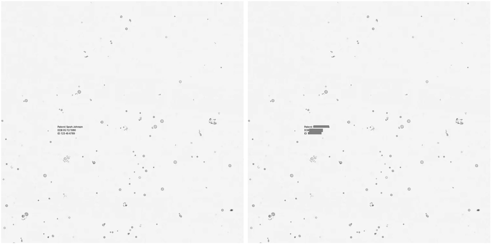
For display DICOM files, present function display_dicom. We can limit the number of files and the number of frames, and enable show metadata:

display_dicom(dicom_df, "content", limit=1, show_meta=True, limit_frame=2)

As shown in the image above, the DICOM frames and metadata are displayed.

Next, we use DicomToImageV3 to extract images from the pixel and overlay data. It returns the results as a Spark DataFrame following Visual NLP’s Image structure.

dicom_to_image = DicomToImageV3() \
    .setInputCols(["content"]) \
    .setOutputCol("image_raw") \
    .setKeepInput(True)

Step 2 – Running Visual NLP Pipelines for PHI Detection in WSI Tiles

To identify which tiles contain PHI, we use a text detection pipeline:

bin_to_image = BinaryToImage() \
    .setInputCol("content") \
    .setOutputCol("image_raw") \
    .setImageType(ImageType.TYPE_BYTE_GRAY) \
    .setKeepInput(False)

text_detector = ImageTextDetector.pretrained("image_text_detector_mem_opt", "en", "clinical/ocr") \
    .setInputCol("image_raw") \
    .setOutputCol("text_regions") \
    .setScoreThreshold(0.7) \
    .setLinkThreshold(0.5) \
    .setWithRefiner(True) \
    .setTextThreshold(0.4) \
    .setSizeThreshold(-1) \
    .setUseGPU(True) \
    .setWidth(0)

pipeline = PipelineModel(stages=[bin_to_image, text_detector])
result = pipeline.transform(image_df)

Only tiles with detected text are passed to the next stage — saving compute and time.

from pyspark.sql.functions import size
result = result.filter(size(result["text_regions"]) > 0).cache()
display_images(result, "image_raw")

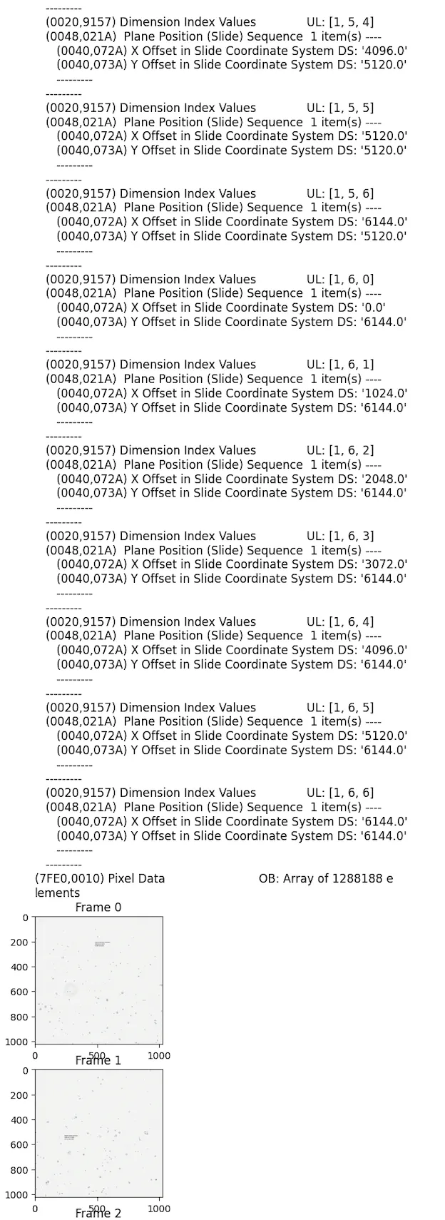
De-identifying PHI from Images

As you can see, the image contains a name, a date of birth, and an ID — all of which are considered PHI (Protected Health Information).

Now apply the actual de-identification pipeline:

from sparkocr.pretrained import PretrainedPipeline
deid_pipeline = PretrainedPipeline("image_deid_multi_model_context_pipeline_cpu", "en", "clinical/ocr")

Let’s run it:

result_deid = deid_pipeline.transform(result)
deid_info = result_deid.select("path", "coordinates").distinct()

And show some results:

deid_info.distinct().show(5, False)

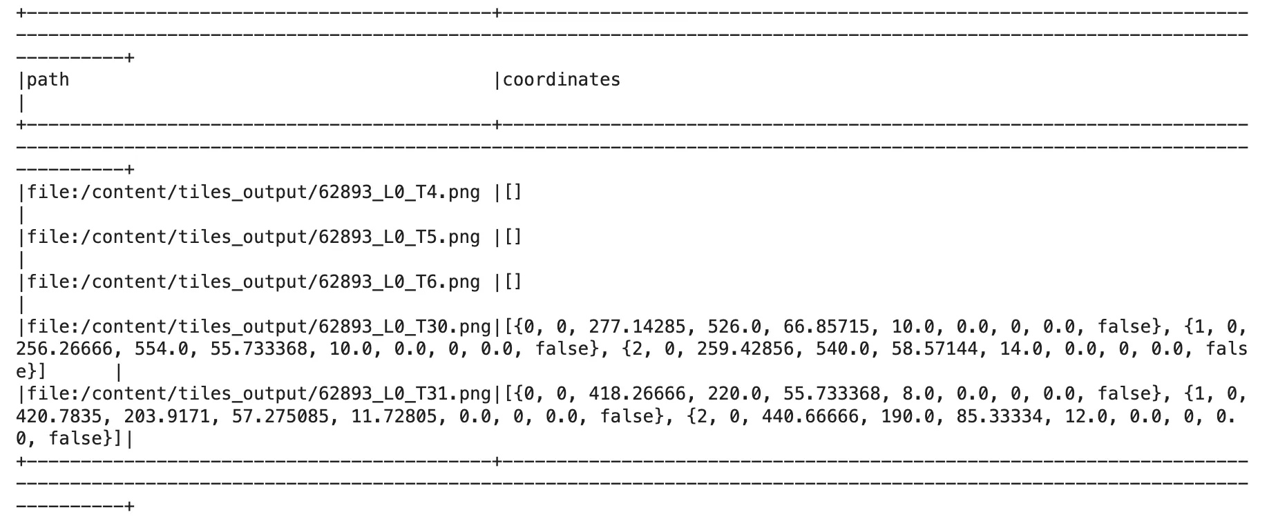
As shown in the previous DataFrame, we return two columns: one containing the file path, and the other with the coordinates of the bounding boxes where PHI was detected.

Cache the results:

We can cache the regions to disk to avoid unnecessary re-computation and to make it easier to recover in case something fails.

deid_info.repartition(10).write.format("parquet").mode("overwrite").save("./cached_regions.parquet")
deid_info = spark.read.parquet("./cached_regions.parquet").repartition(10)

Visual check:

from sparkocr.utils import display_images
display_images(result_deid, "image_with_regions")

As shown in the image above, the PHI regions have been redacted by overlaying black bounding boxes.

Step 3 – Reconstructing and Saving PHI-Free SVS and DICOM Clean Outputs

3.1. For SVS:

This is the final step! We now mask the specific tiles in the source SVS file using the PHI regions detected earlier. Since SVS files use a pyramid of image resolutions, redactions applied at the selected level are automatically scaled across all levels for consistency.

from sparkocr.utils.svs.phi_redaction import redact_phi_in_tiles
redact_phi_in_tiles("deid_svs_copy", deid_info, OUTPUT_FOLDER, output_svs_path=svs_path_out, create_new_svs_file = True)

The output will be a clean SVS file with all detected PHI removed — across image tiles, auxiliary images, and metadata. This de-identified file is now safe for use in research, AI model training, or secure data sharing.

A notebook with a full example can be found here.

3.2. For Dicom:

We draw and redact PHI regions directly on DICOM tiles using two transformers:

draw_regions = DicomDrawRegions() \
    .setInputCol("content") \
    .setInputRegionsCol("coordinates") \
    .setOutputCol("dicom") \
    .setAggCols(["path", "content"]) \
    .setKeepInput(True)

dicom_deidentifier = DicomMetadataDeidentifier() \
    .setInputCols(["dicom"]) \
    .setOutputCol("dicom_cleaned")\
    .setKeepInput(True)

• DicomDrawRegions: draw regions on top of the frames. We will be masking both pixel and overlay data.
• DicomMetadataDeidentifier: this transformer will de-indentify the metadata.

Inspect Intermmediate Stages

display_dicom(result_clean, "content, dicom_cleaned")

Below is an excerpt comparing the DICOM file before and after de-identification:

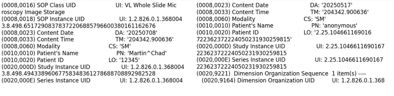
As seen in the image above, the Patient Name has been de-identified by replacing it with the placeholder “anonymous”. Other DICOM tags have also been redacted.

Save clean files:

The final step in this post is saving the result back as a DICOM file on disk. To preserve the original filenames, we first define a UDF to extract the file name from the path column:

def get_name(path, keep_subfolder_level=0):
    path = path.split("/")
    path[-1] = path[-1].split('.')[0]
    return "/".join(path[-keep_subfolder_level-1:])

To save the cleaned DICOM files using the binaryFormat data source, specify the file type (dicom), the DataFrame field containing the file, a filename prefix, the nameField column, and the target outputPath.

from pyspark.sql.functions import *

output_path = "./../data/dicom/deidentified/"

result.withColumn("fileName", udf(get_name, StringType())(col("path"))) \
    .write \
    .format("binaryFormat") \
    .option("type", "dicom") \
    .option("field", "dicom_cleaned") \
    .option("prefix", "ocr_") \
    .option("nameField", "fileName") \
    .mode("overwrite") \
    .save(output_path)

Load back for inspection:

After saving, we can load the cleaned DICOM files to verify the results:

dicom_gen_df = spark.read.format("binaryFile").load("./../data/dicom/deidentified/*.dcm")
display_dicom(dicom_gen_df)

You can find the Jupyter notebook with the full code here.

Coming soon: Learn how to deploy this as a scalable API on AWS SageMaker in Part 3.

Summary

End-to-End PHI Removal in SVS and DICOM with Visual NLP

In this post, we:

• Stripped Protected Health Information (PHI) from SVS and DICOM formats to ensure regulatory compliance

• Automatically detected and redacted text-based PHI within image tiles using clinical NLP

• Reconstructed anonymized, high-fidelity files ready for safe and compliant downstream use

What’s Next?

In Part 3, we’ll deploy this pipeline as a cloud-based API using AWS SageMaker, turning this process into a scalable and production-ready service.

Resources

• Visual NLP SVS De-Identification Notebook
• Visual NLP Dicom De-Identification Notebook
• WSI Dataset
• Visual NLP Workshop

FAQ

What is the goal of de-identifying SVS and DICOM WSI files?
The goal is to remove Protected Health Information (PHI) from whole slide images, both from metadata and image content, to ensure compliance with HIPAA, GDPR, and to enable safe use in AI and research.

How does Visual NLP process PHI in SVS files?
It removes metadata and auxiliary images containing PHI, extracts tiles for text detection, identifies redaction zones, and reconstructs a clean SVS file with consistent masking across all image levels.

How is PHI detected in image tiles?
Visual NLP uses an OCR-based text detection pipeline to identify text regions. Only tiles with detected text are passed to the de-identification model, optimizing processing time.

Can Visual NLP handle PHI in DICOM images?
Yes, Visual NLP extracts pixel and overlay data from DICOM frames, detects PHI, masks visual data, and de-identifies sensitive metadata to produce compliant files.

What output formats are supported after de-identification?
Clean SVS and DICOM files are saved in their respective formats. Redacted image regions and metadata are reconstructed to preserve file structure and allow downstream analysis.

Is the de-identification process scalable?
Yes, the pipeline supports multi-threading, caching, and can be deployed as an API using platforms like AWS SageMaker for scalable, production-grade applications.

Who should use this Visual NLP pipeline?
This solution is ideal for digital pathology teams, healthcare AI developers, compliance officers, and researchers working with high-resolution whole slide images in clinical workflows.