


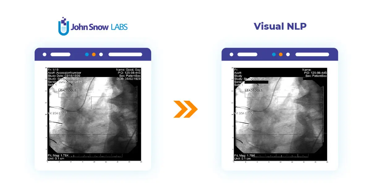
Start to work with DICOM in Visual NLP
In this post, we are deeply diving into working with metadata using Visual NLP.
We are going to make use of Visual NLP pipelines. Visual NLP pipelines are Spark ML pipelines. Each stage(a.k.a ‘transformer’) in the pipeline is in charge of a specific task. We will make use of these two Visual NLP transformers in the following example,
- DicomToMetadata: this transformer will extract metadata from the DICOM document.
- DicomMetadataDeidentifier: this transformer will de-indentify the metadata.
To start, you need to read DICOM files into the data frame using the binaryFile data source of Spark:
dicom_df = spark.read.format("binaryFile").load(dicom_path)
dicom_df.show()
+--------------------+-------------------+-------+--------------------+
| path| modificationTime| length| content|
+--------------------+-------------------+-------+--------------------+
|file:/Users/nmeln...|2023-08-20 14:17:23|1049988|[52 75 62 6F 20 4...|
|file:/Users/nmeln...|2023-08-20 14:17:23| 651696|[00 00 00 00 00 0...|
|file:/Users/nmeln...|2023-08-20 14:17:23| 640574|[00 00 00 00 00 0...|
|file:/Users/nmeln...|2023-08-20 14:17:23| 426776|[52 75 62 6F 20 4...|
+--------------------+-------------------+-------+--------------------+
First, we can check the number of files and size. Dicom documents can have sizes from a few kilobytes to a few gigabytes.
dicom_df.select(f.col("length") / 2**20).summary().show()
+-------+-------------------+
|summary| (length / 1000000)|
+-------+-------------------+
|  count|                  3|
|   mean| 0.7057793333333332|
| stddev|0.31668138697645826|
|    min|           0.426776|
|    25%|           0.426776|
|    50%|           0.640574|
|    75%|           1.049988|
|    max|           1.049988|
+-------+-------------------+
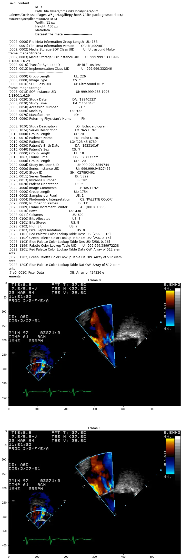
For display DICOM files, present function display_dicom. We can limit the number of files and the number of frames, and enable show metadata:
display_dicom(dicom_df, "content", limit=1, show_meta=True, limit_frame=2)
DicomToMetadata
DicomToMetadata transformer helps to extract metadata to the data frame column as JSON:
dicom = DicomToMetadata() \
   .setInputCol("content") \
   .setOutputCol("metadata")

result = dicom.transform(dicom_df)
result.show()
+--------------------+-------------------+-------+--------------------+
|                path|   modificationTime| length|            metadata|
+--------------------+-------------------+-------+--------------------+
|file:/Users/nmeln...|2023-08-20 14:17:23|1049988|{\n    "SpecificC...|
|file:/Users/nmeln...|2023-08-20 14:17:23| 651696|{\n    "ImageType...|
|file:/Users/nmeln...|2023-08-20 14:17:23| 640574|{\n    "StudyDate...|
|file:/Users/nmeln...|2023-08-20 14:17:23| 426776|{\n    "GroupLeng...|
+--------------------+-------------------+-------+--------------------+
Let’s read it as the JSON using spark capabilities and use pandas for prettify results:
# Import the necessary functions
from pyspark.sql.functions import from_json
# Get the schema of the 'metadata' column (present as a string with JSON in the
# result DataFrame)
json_schema = spark.read.json(result.rdd.map(lambda row: row.metadata)).schema
# Convert the 'metadata' column to a struct using the 'from_json' function
metadata = result.select(from_json('metadata', json_schema).alias("metadata"))
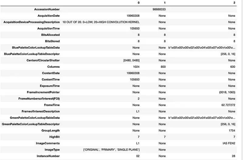
# Select all subfields and convert them to a Pandas DataFrame, then transpose it
metadata.select("metadata.*").toPandas().T
To understand the actual size of the data that we have, we need to check the related number of frames in the dataset:
metadata.select(f.col("metadata.NumberofFrames").alias("NumberOfFrames").cast("int")) \
  .na.fill(1).summary()
+-------+--------------+
|summary|NumberOfFrames|
+-------+--------------+
|  count|             4|
|   mean|           3.5|
| stddev|           5.0|
|    min|             1|
|    25%|             1|
|    50%|             1|
|    75%|             1|
|    max|            11|
+-------+--------------+
And get the total number of frames using aggregation:
metadata.select(f.col("metadata.NumberofFrames").alias("NumberOfFrames").cast("int").alias("frames")) \
 .fillna(1) \
 .groupBy() \
 .sum()
Output: 13
Another useful characteristic of the dataset is the resolution of images. So, let’s extract the width of the pixel data and calculate statistics:
metadata.select(f.col("metadata.Rows").alias("width").cast("int")).summary()
+-------+-----------------+
|summary|            width|
+-------+-----------------+
|  count|                4|
|   mean|            657.5|
| stddev|308.5595566499278|
|    min|              376|
|    25%|              376|
|    50%|              430|
|    75%|              800|
|    max|             1024|
+-------+-----------------+
We can group by and aggregate by any metadata tag, for example, PhotometricInterpretation:
metadata.select(f.col("metadata.PhotometricInterpretation")) \
 .groupBy("PhotometricInterpretation") \
 .count()
+-------------------------+-----+
|PhotometricInterpretation|count|
+-------------------------+-----+
|              MONOCHROME2|    3|
|            PALETTE COLOR|    1|
+-------------------------+-----+
All these statistics of the dataset allow us to analyze the dataset and calculate how many resources we need to have to process the dataset.
Jupyter Notebook with full code can be found here.
DicomMetadataDeidentifier
DicomMetadataDeidentifier helps to de-identify metadata of DICOM files in Visual NLP. It cleaned tags that can contain PHI.
dicom_deidentifier = DicomMetadataDeidentifier() \
  .setInputCols(["content"]) \
  .setOutputCol("dicom_cleaned")

result = dicom_deidentifier.transform(dicom_df)

result.show()
+--------------------+---------+--------------------+-------------------+-------+
|       dicom_cleaned|exception|                path|   modificationTime| length|
+--------------------+---------+--------------------+-------------------+-------+
|[52 75 62 6F 20 4...|         |file:/Users/nmeln...|2023-08-20 14:17:23|1049988|
|[00 00 00 00 00 0...|         |file:/Users/nmeln...|2023-08-20 14:17:23| 651696|
|[00 00 00 00 00 0...|         |file:/Users/nmeln...|2023-08-20 14:17:23| 640574|
|[52 75 62 6F 20 4...|         |file:/Users/nmeln...|2023-08-20 14:17:23| 426776|
+--------------------+---------+--------------------+-------------------+-------+
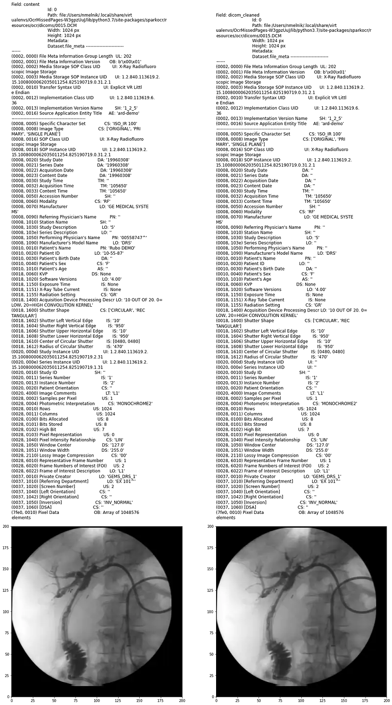
To compare the original metadata and cleaned, let’s add keepInput to the DicomMetadataDeidentifier and display results using display_dicom:
dicom_deidentifier = DicomMetadataDeidentifier() \
 .setInputCols(["content"]) \
 .setOutputCol("dicom_cleaned") \
 .setKeepInput(False)

result = dicom_deidentifier.transform(dicom_df)

display_dicom(result, "content,dicom_cleaned")
In the next post, we will work with pixel data.