


Converting tables in scanned documents & images into structured data
Motivation
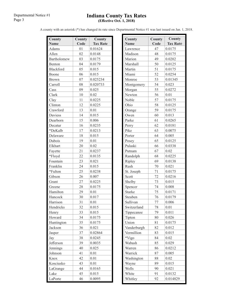
Extracting data formatted as a table is a common task – whether you’re analyzing financial statements, academic research papers, or clinical trial documentation. For example, assume that you’re given this example document, with a page showing tax rates per county, and need to code a program that calculates taxes using those rates. Your first step will be to get the table out of this human-readable document (handling the formatting, layout, and the fact that it’s actually two side-by-side tables) into a computer-readable one (such as a Python data frame or a relational data table).
The difficulty of this task depends on how the document you were given is formatted. If it is a PDF or DOCX document with digital text – meaning that the structured data is stored in the file, along with formatting on how to display it – then extracting the tabular data is a matter of “reverse engineering” it from the file. Spark OCR – a commercial software library for state-of-the-art visual document understanding from John Snow Labs – has built-in support to get this done:
- Jupyter notebook: Extract data from selectable tables in PDF files
- Jupyter notebook: Extract data from selectable tables in DOCX files
However, this task becomes harder if the table is simply an image. This happens if the original table was scanned, faxed, photographed, or simply copy & pasted as a picture in the document you received. In this case, the structured data is not in the file and needs to be extracted using computer vision and object character recognition.
Fortunately, Spark NLP OCR includes out-of-the-box algorithms and pre-trained models to make this possible. The rest of this post explains how to put together an end-to-end automated pipeline with the three subtasks this challenge is composed of:
- Detect tables in an image
- Detect cells within a visual table
- Recognize text within each cell
The Example of Spark OCR for Table Detection & Extraction Jupyter Notebook is public so that you can run the end-to-end solution yourself. Note that in the code, the tables are read as JPG files, but if your documents include images as part of PDF or DOCX files, this requires only one additional step in the Spark OCR pipeline.
In order to run the code, you will need a Spark OCR license, for which a 30-day free trial is available here. Spark OCR runs on your infrastructure – your data is never sent to John Snow Labs or any other third party. You can run the software on your laptop, on a server, or at scale on a Spark cluster.
Detect tables in an image
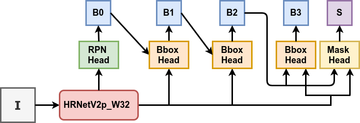
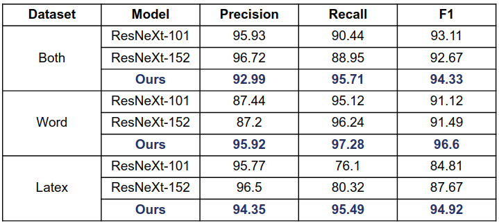
For table detection, Spark OCR has ImageTableDetector. It is an object detection deep learning model, inspired by CascadeTabNet which uses a Cascade mask Region-based CNN High-Resolution Network (Cascade mask R-CNN HRNet).
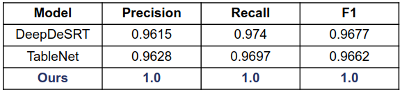
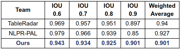
The out-of-the-box model was pre-trained on the COCO dataset and fine-tuned on the ICDAR 2019 competition dataset for table detection. It demonstrates the state of the art results for ICDAR 2013 and TableBank, and top results for ICDAR 2019:
ICDAR 2013
ICDAR 19 (Track A Modern)
TableBank
Let’s read the image to the data frame using BinaryToImage, call ImageTableDetector and draw detected regions to the original image using ImageDrawRegions:
        image_df = spark.read.format("binaryFile").load(imagePath)binary_to_image = BinaryToImage()
        binary_to_image.setImageType(ImageType.TYPE_3BYTE_BGR)table_detector = ImageTableDetector \
            .pretrained("general_model_table_detection_v2", "en", "clinical/ocr") \
            .setInputCol("image") \
            .setOutputCol("table_regions")draw_regions = ImageDrawRegions() \
            .setInputCol("image") \
            .setInputRegionsCol("table_regions") \
            .setOutputCol("image_with_regions")pipeline = PipelineModel(stages=[
            binary_to_image,
            table_detector,
            draw_regions
        ])result =  pipeline.transform(image_df)
        display_images(result, "image_with_regions")
There is output for the pipeline:
Detect cells within a visual table
Our second computer vision task is to detect the individual cells within each table. Cell detection is implemented in the ImageCellDetector transformer. It is based on image processing algorithms that detect horizontal and vertical lines.
Before calling ImageCellDetector, we need first to extract the table images from the main image. The ImageSplitRegions transformer will help us here. To improve the accuracy of text recognition, we can also scale table images using the ImageScaler – note that all the image enhancement algorithms implemented within Spark OCR are at your disposal at this point:
        splitter = ImageSplitRegions() \
        .setInputCol("image") \
        .setInputRegionsCol("region") \
        .setOutputCol("table_image") \
        .setDropCols("image") \
        .setImageType(ImageType.TYPE_BYTE_GRAY)
    scaler = ImageScaler() \
        .setInputCol("table_image") \
        .setOutputCol("scaled_image") \
        .setScaleFactor(2)
    cell_detector = ImageTableCellDetector() \
        .setInputCol("scaled_image") \
        .setOutputCol("cells") \
        .setKeepInput(True)
    pipeline = PipelineModel(stages=[
        binary_to_image,
        table_detector,
        splitter,
        scaler,
        cell_detector,
    ])
    result =  pipeline.transform(image_df)
    results.show(1, False)
The output contains an array of cells’ coordinates:
        +----------------------------------------------------------+
        | cells                                                    |
        +----------------------------------------------------------+
        |[[[[11, 15, 168, 62]], [[181, 15, 112, 62]],              |
        |[[295, 15, 140, 62]]], [[[11, 80, 168, 33]],              |
        |[[181, 80, 112, 33]], [[295, 80, 140, 33]]],              |
        |[[[11, 115, 168, 34]], [[181, 115, 112, 34]],             |
        |[[295, 115, 140, 34]]], [[[11, 151, 168, 34]],            |
        |[[181, 151, 112, 34]], [[295, 151, 140, 34]]],            |
        |[[[11, 187, 168, 34]], [[181, 187, 112, 34]],             |
        |[[295, 187, 140, 3 ...                                    |
        +----------------------------------------------------------+
Recognize text within each cell
The last step in our pipeline is the ImageCellsToTextTable transformer. It uses OCR to recognize and extract text from each detected cell, and return all that extracted text in a single data frame:
        table_recognition = ImageCellsToTextTable()
        table_recognition.setInputCol("scaled_image")
        table_recognition.setCellsCol('cells')
        table_recognition.setMargin(1)
        table_recognition.setStrip(True)
        table_recognition.setOutputCol('table')
Let’s assemble the whole pipeline which contains all needed transformers and call it:
        pipeline = PipelineModel(stages=[
        binary_to_image,
        table_detector,
        splitter,
        scaler,
        cell_detector,
        table_recognition
    ])
    results = pipeline.transform(image_df).cache()
    results.select("table").collect()[0]
Output:
        +------------------------------------------------------------------+
        |table                                                             |
        +------------------------------------------------------------------+
        |[[0, 0, 0.0, 0.0, 444.0, 1744.0], [[[CountyName, 11.0, 15.0, 168.0|
        |, 62.0], [CountyCode, 181.0, 15.0, 112.0, 62.0], [CountyTax Rate, |
        |295.0, 15.0, 140.0, 62.0]], [[Lawrence, 11.0, 80.0, 168.0, 33.0], |
        |[47, 181.0, 80.0, 112.0, 33.0], [0.0175, 295.0, 80.0, 140.0,      |
        |33.0]], [[Madison, 11.0, 115.0, 168.0, 34.0], [48, 181.0, 115.0,  |
        |112.0, 34.0], [0.0175, 295.0, 115.0, 140.0, 34.0]], [[Marion, 11.0|
        |, 151.0, 168.0, 34.0], [49, 181.0, 151.0, 112.0, 34.0], [0.0202,  |
        |295.0, 151.0, 140.0, 34.0]], [[Marshall, 11.0, 187.0, 168.0, 34.0]|
        |, [50, 181.0, 187.0, 112.0, 34.0], [0.0125, 295.0, 187.0, 140.0,  |
        |34.0]], [[Martin, 11.0, 223.0, 168.0, 34.0], [S51, 181.0, 223.0,  |
        |112.0, 34.0], [0.0175, 295.0, 223.0, 1 ...                        |
        +------------------------------------------------------------------+
To display the tabular data as a data frame, we can explore the output structure and add a table column with an index of the table on the page:
exploded_results = results.select("table", "region") \
        .withColumn("cells", f.explode(f.col("table.chunks"))) \
        .select([f.col("filename"), f.col("region.index").alias("table")] + [f.col("cells")[i].getField("chunkText").alias(f"col{i}") for i in
                 range(0, 3)]) \
    exploded_results.show(100, False)
As the result we have:
        +----------------+-----+-----------+----------+--------------+
        |filename        |table|col0       |col1      |col2          |
        +----------------+-----+-----------+----------+--------------+
        |cTDaR_t10011.jpg|0    |CountyName |CountyCode|CountyTax Rate|
        |cTDaR_t10011.jpg|0    |Lawrence   |47        |0.0175        |
        |cTDaR_t10011.jpg|0    |Madison    |48        |0.0175        |
        |cTDaR_t10011.jpg|0    |Marion     |49        |0.0202        |
        |cTDaR_t10011.jpg|0    |Marshall   |50        |0.0125        |
        |cTDaR_t10011.jpg|0    |Martin     |S51       |0.0175        |
        |cTDaR_t10011.jpg|0    |Miami      |52        |0.0254        |
        |cTDaR_t10011.jpg|0    |Monroe     |53        |0.01345       |
        |cTDaR_t10011.jpg|0    |Montgomery |54        |0.023         |
        |cTDaR_t10011.jpg|0    |Morgan     |55        |0.0272        |
        |cTDaR_t10011.jpg|0    |Newton     |56        |0.01          |
        |cTDaR_t10011.jpg|0    |Noble      |57        |0.0175        |
        |cTDaR_t10011.jpg|0    |Ohio       |58        |0.0125        |
        |cTDaR_t10011.jpg|0    |Orange     |59        |0.0175        |
        |cTDaR_t10011.jpg|0    |Owen       |60        |0.013         |
        |cTDaR_t10011.jpg|0    |Parke      |61        |0.0265        |
        |cTDaR_t10011.jpg|0    |Perry      |62        |O.O181        |
        |cTDaR_t10011.jpg|0    |Pike       |63        |0.0075        |
        |cTDaR_t10011.jpg|0    |Porter     |64        |0.005         |
        |cTDaR_t10011.jpg|0    |Posey      |65        |0.0125        |
        |cTDaR_t10011.jpg|0    |Pulaski    |66        |0.0338        |
        |cTDaR_t10011.jpg|0    |Putnam     |67        |0.02          |
        |cTDaR_t10011.jpg|0    |Randolph   |68        |0.0225        |
        |cTDaR_t10011.jpg|0    |Riplev     |69        |0.0138        |
        |cTDaR_t10011.jpg|0    |Rush       |70        |0.021         |
        |cTDaR_t10011.jpg|0    |St. Joseph |71        |0.0175        |
        |cTDaR_t10011.jpg|0    |Scott      |72        |0.0216        |
        |cTDaR_t10011.jpg|0    |Shelby     |73        |0.015         |
        |cTDaR_t10011.jpg|0    |Spencer    |74        |0.008         |
        |cTDaR_t10011.jpg|0    |Starke     |75        |0.0171        |
        |cTDaR_t10011.jpg|0    |Steuben    |76        |0.0179        |
        |cTDaR_t10011.jpg|0    |Sullivan   |77        |0.006         |
        |cTDaR_t10011.jpg|0    |Switzerland|78        |0.01          |
        |cTDaR_t10011.jpg|0    |Tippecanoe |79        |0.011         |
        |cTDaR_t10011.jpg|0    |Tipton     |80        |0.026         |
        |cTDaR_t10011.jpg|0    |Union      |R81       |0.0175        |
        |cTDaR_t10011.jpg|0    |Vanderburgh|&2        |0.012         |
        |cTDaR_t10011.jpg|0    |Vermillion |83        |0.015         |
        |cTDaR_t10011.jpg|0    |*Vigo      |&4        |0.02          |
        |cTDaR_t10011.jpg|0    |Wabash     |&5        |0.029         |
        |cTDaR_t10011.jpg|0    |Warren     |86        |0.0212        |
        |cTDaR_t10011.jpg|0    |Warrick    |87        |0.005         |
        |cTDaR_t10011.jpg|0    |Washineton |88        |0.02          |
        |cTDaR_t10011.jpg|0    |Wayne      |go        |0.015         |
        |cTDaR_t10011.jpg|0    |Wells      |90        |0.021         |
        |cTDaR_t10011.jpg|0    |White      |91        |0.0132        |
        |cTDaR_t10011.jpg|0    |Whitley    |9?        |0.014829      |
        |cTDaR_t10011.jpg|1    |CountyName |CountyCode|CountyTax Rate|
        |cTDaR_t10011.jpg|1    |Adams      |ol        |0.01624       |
        |cTDaR_t10011.jpg|1    |Allen      |02        |0.0148        |
        |cTDaR_t10011.jpg|1    |Bartholomew|03        |0.0175        |
        |cTDaR_t10011.jpg|1    |Benton     |04        |0.0179        |
        |cTDaR_t10011.jpg|1    |Blackford  |os        |0.015         |
        |cTDaR_t10011.jpg|1    |Boone      |06        |0.015         |
        |cTDaR_t10011.jpg|1    |Brown      |07        |0.025234      |
        |cTDaR_t10011.jpg|1    |Carroll    |og        |0.020733      |
        |cTDaR_t10011.jpg|1    |Cass       |09        |0.025         |
        |cTDaR_t10011.jpg|1    |Clark      |10        |0.02          |
        |cTDaR_t10011.jpg|1    |Clay       |ll        |0.0225        |
        |cTDaR_t10011.jpg|1    |Clinton    |12        |0.0225        |
        |cTDaR_t10011.jpg|1    |Crawford   |13        |0.01          |
        |cTDaR_t10011.jpg|1    |Daviess    |14        |0.015         |
        |cTDaR_t10011.jpg|1    |Dearborn   |15        |0.006         |
        |cTDaR_t10011.jpg|1    |Decatur    |16        |0.0235        |
        |cTDaR_t10011.jpg|1    |*DeKalb    |17        |0.0213        |
        |cTDaR_t10011.jpg|1    |Delaware   |18        |0.015         |
        |cTDaR_t10011.jpg|1    |Dubois     |19        |0.01          |
        |cTDaR_t10011.jpg|1    |Elkhart    |20        |0.02          |
        |cTDaR_t10011.jpg|1    |Favette    |21        |0.0237        |
        |cTDaR_t10011.jpg|1    |*Floyd     |22        |0.0135        |
        |cTDaR_t10011.jpg|1    |Fountain   |23        |0.021         |
        |cTDaR_t10011.jpg|1    |Franklin   |24        |0.015         |
        |cTDaR_t10011.jpg|1    |*Fulton    |25        |0.0238        |
        |cTDaR_t10011.jpg|1    |Gibson     |26        |0.007         |
        |cTDaR_t10011.jpg|1    |Grant      |27        |0.0225        |
        |cTDaR_t10011.jpg|1    |Greene     |28        |0.0175        |
        |cTDaR_t10011.jpg|1    |Hamilton   |29        |0.01          |
        |cTDaR_t10011.jpg|1    |Hancock    |30        |0.017         |
        |cTDaR_t10011.jpg|1    |Harrison   |31        |0.01          |
        |cTDaR_t10011.jpg|1    |Hendricks  |32        |0.015         |
        |cTDaR_t10011.jpg|1    |Henry      |33        |0.015         |
        |cTDaR_t10011.jpg|1    |Howard     |34        |0.0175        |
        |cTDaR_t10011.jpg|1    |Huntington |35        |0.0175        |
        |cTDaR_t10011.jpg|1    |Jackson    |36        |0.021         |
        |cTDaR_t10011.jpg|1    |Jasper     |37        |0.02864       |
        |cTDaR_t10011.jpg|1    |Jay        |38        |0.0245        |
        |cTDaR_t10011.jpg|1    |Jefferson  |39        |0.0035        |
        |cTDaR_t10011.jpg|1    |Jennings   |40        |0.025         |
        |cTDaR_t10011.jpg|1    |Johnson    |41        |0.01          |
        |cTDaR_t10011.jpg|1    |Knox       |42        |0.01          |
        |cTDaR_t10011.jpg|1    |Kosciusko  |43        |0.01          |
        |cTDaR_t10011.jpg|1    |LaGrange   |44        |0.0165        |
        |cTDaR_t10011.jpg|1    |Lake       |45        |0.015         |
        |cTDaR_t10011.jpg|1    |LaPorte    |46        |0.0095        |
        +----------------+-----+-----------+----------+--------------+
The current implementation of the ImageCellDetector supports only tables with borders and white background. We are working to expand support to borderless tables, dark & noisy backgrounds, uncommon table layouts, multilingual text, and international number & currency formats. Please contact us if you have challenging documents or images that you’d like us to support.
Links
- Jupyter Notebook: Using Spark OCR for Table Detection & Extraction
- Additional Spark OCR Examples: Spark OCR Workshop
- CascadeTabNet: An approach for an end to end table detection and structure recognition from image-based documents
- Spark OCR Documentation
- PDF OCR