Scaling John Snow Labs Medical LLMs on Databricks environments

Previously, we described how to deploy modern visual LLMs on Databricks environments at Deploying John Snow Labs Medical LLMs on Databricks: Three Flexible Deployment Options. Available options are flexible enough to fit almost any requirements in terms of available environment. Real-life use cases pose additional challenges:

• Pipelines may include heterogeneous calculations that require different loads on CPU and GPU.
• Load may fluctuate, let’s say intensive load during working hours and low or no load during night time.

Assigning cluster size, endpoint concurrency or nodes’ types on max load may not be optimal in terms of cost or even too expensive. Here, we address these issues and explain how to scale John Snow Labs Medical LLMs on Databricks environments

Scaling Visual LLMs

In the article mentioned above we listed 3 ways of deployment on Databricks environment. We saw three deployment options:

• General purpose cluster
• Container Service
• Model Serving

The case of general purpose cluster is pretty common and well known by the community. Today we are focusing on the other two options.

Container services

The cluster of containers is very similar to your usual cluster. Actually, it is still a general purpose cluster. You are still able to leverage Databrick’s autoscaling for cluster size to increase or to reduce the number of workers according to the volume of your input workload.

When load grows, Databricks will add more nodes, when load decreases, nodes will be released. This feature shines when you have a fluctuating load of input documents. It is well-known that Visual LLMs require powerful and expensive GPUs, it may be very expensive to maintain a cluster size that matches the max load which could happen during a short period of time. With our Docker images that allow for scalability, it is possible to save significantly on infrastructure cost.

Numbers speak by themselves: after the initial tuning process we were able to reach a throughput of 6 sec/image to extract complex structured data from handwritten text. It is 10 one-page documents per minute, 600 one-page documents per hour on one node. It is faster, cheaper, and more manageable than using LLM from API providers. Under this scalability regime, you can process almost any workload.

The weak point of this approach is applying it for pipelines that include a significant part of CPU calculations along with GPU calculations. When a pipeline works on CPU, GPU is idle, it is not used, but it must be paid for. And vice versa. It is better to keep all calculation power busy and working. One way to optimize this is to split the pipeline in two parts, with each part working on separate clusters — one with CPU nodes and another one with a GPU node. Another way is to use a Model Serving endpoint. In this case, the cluster is composed of CPU nodes only, and GPU calculations are delegated/sent to a Model Serving endpoint. Now, let’s jump to Model Serving.

Model serving

John Snow Labs provides LLM distributions for use with Databrick Model Serving technology (contact us to get access for trial usage or demo). Databricks Model Serving is a cutting edge deployment technology, and we encourage you to read more at its Databricks page. In this article, we will just scratch the surface.

When deployed on Databricks Model Serving JSL’s Visual LLM access is provided as an endpoint. While the remaining transformers in the pipeline work on a general purpose cluster composed of CPU nodes only.

In order to connect these two components, i.e., the Spark Pipeline and the Model Serving endpoint, a custom transformer in the Spark Pipeline calls the endpoint to get Visual LLM answers and injects it[them] into the pipeline for further processing. In this way, GPU and CPU parts are separated, and deployed in the best possible way, with each part having their own settings to meet their requirements.

Now, let’s get our hands dirty! First, when you configure a Model Serving endpoint you should put attention on the following points that affect performance:

• Concurrency
• Number of GPU cards available to compute type

This is what it looks on the Databrics interface:

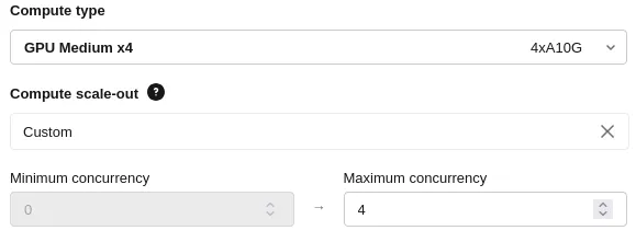
Please note that term concurrency is not roughly mapped on to nodes. Instead, it controls how many simultaneous requests your endpoint can process, refer to Databricks documentation to get more information.

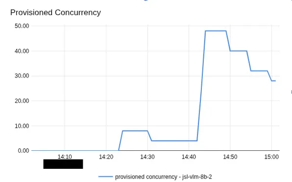
You should be aware that scaling from zero to desired size may take some time, up to 10–15 mins to warm up. During that time frame, the endpoint will return an error status code. It is better to anticipate this behavior at your pipeline a step that wakes up the endpoint in advance — send a dummy request to the endpoint, it wakes up, then start sending real workload.

Other considerations

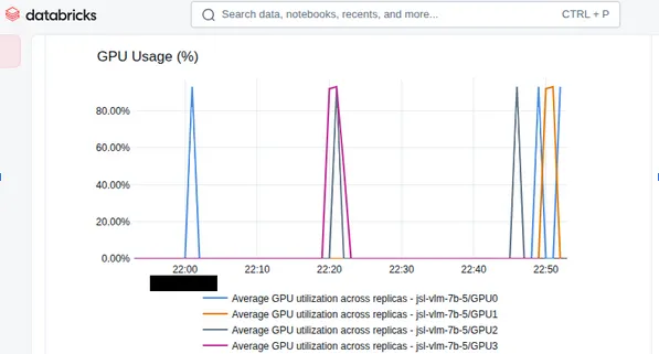
Regarding the number of GPU cards. More cards does not always result in more performance. To get the most out of it, you need to set up the client side in the pipeline appropriately. Fortunately, Databricks provides a good tool to monitor load. For example, in the GPU Usage metrics below you may see that although there are 4 GPU cards, only 2 of them are being used. So, for this load there is no need to pay for these two extra cards.

Lessons learned

Key take-aways from these evaluations are as follows:

• Look after metrics (especially GPU Usage)
• Put attention on setting up the client part to get the most

During set up of the client part you should put attention on the following:

• Sending images to process by batches definitely improves performance. Larger batch size is better. But you should be aware of limitations. Since data is sent via HTTP Post method its payload is limited so you can not increase batch size indefinitely. Actual max size depends on sizes of your input documents. Roughly, batch size equals max payload size divided by average image size.
• Increasing the size of the cluster that calls the endpoint may also increase load and improve performance, but it increases spendings as well.

In summary, you need find the best balance between:

• Endpoint concurrency capacity.
• Number of GPU cards.
• Cluster size.
• Budget.

John Snow Labs’ models on Databricks Model Serving endpoints is a very flexible way to fulfill many different requirements. For some projects, we were able to get 3 sec/image for complex data extraction using it.

Environment

A few words about environments that were used when we got performance results:

• Node types for Container Service cluster were with A100 or H100 GPUcards.
• Compute types for Model Serving endpoints were with A100 GPU cards
• Images were about 960×1280 dimensionality, ~ 0.9–1.5 MB size.

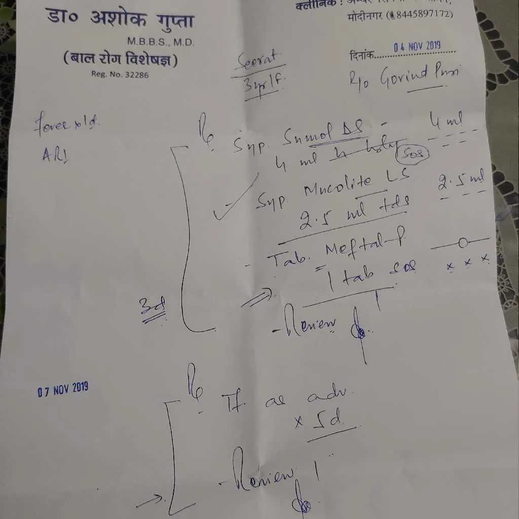
Below are samples of input data from publicly available dataset. One real page of the document may contain several medicines records along with patient and doctor data.

Comparison

Both options are pretty flexible and give the ability to process variable loads smoothly. Though there are a few advantages for each option.

Container Service’s salient features are:

• Passing data to Visual LLM via memory. Because Spark already takes care of data distribution, no requests with heavy payloads are required. In the case of the endpoint, it is required to send data via HTTP which adds extra load and limitations. Passing data via RAM is always a faster option.
• Wider list of options for node types, more flexibility in selection of required GPU cards and cost.

Model Serving salient features are:

• Natural splitting of CPU and GPU parts.
• Possibility to call endpoints outside of Databricks.

Choose Container Service when:

• You need more performance.
• You need more flexibility in nodes selection

Choose Model Serving when:

• There is significant disbalance in CPU/GPU calculations and you need to split their environments.
• You need to call the scalable GPU environment outside of Databricks.

Conclusion

John Snow Labs provides Visual LLMs that allows you to get the most out of scalable architectures in Databricks. Visual LLMs processing times can be as low as 3–6 sec per image to extract information on one node/replica. You can process hundreds of docs per hour and add more processing power if it is required. With our models, you can accurately process your data with high-performance, and at an affordable price.